Long-range only LODE descriptor
The LodeSphericalExpansion allows the
calculation of a descriptor that includes all atoms within the system and projects them
onto a spherical expansion/ fingerprint within a given cutoff. This is very useful
if long-range interactions between atoms are important to describe the physics and
chemistry of a collection of atoms. However, as stated the descriptor contains ALL
atoms of the system and sometimes it can be desired to only have a long-range/exterior
only descriptor that only includes the atoms outside a given cutoff. Sometimes there
descriptors are also denoted by far-field descriptors.
A long range only descriptor can be particular useful when one already has a good descriptor for the short-range density like (SOAP) and the long-range descriptor (far field) should contain different information from what the short-range descriptor already offers.
Such descriptor can be constructed within rascaline as sketched by the image below.

In this example will construct such a descriptor using the radial integral splining tools of rascaline.
We start the example by loading the required packages
import ase
import ase.visualize.plot
import matplotlib.pyplot as plt
import numpy as np
from ase.build import molecule
from metatensor import LabelsEntry, TensorMap

from rascaline import LodeSphericalExpansion, SphericalExpansion
from rascaline.utils import (
    GaussianDensity,
    LodeDensity,
    LodeSpliner,
    MonomialBasis,
    SoapSpliner,
)
Single water molecule (short range) system
Our first test system is a single water molecule with a \(15\,\mathrm{Å}\) vacuum layer around it.
atoms = molecule("H2O", vacuum=15, pbc=True)
We choose a cutoff for the projection of the spherical expansion and the neighbor
search of the real space spherical expansion.
cutoff = 3
We can use ase’s visualization tools to plot the system and draw a gray circle to
indicate the cutoff radius.
fig, ax = plt.subplots()

ase.visualize.plot.plot_atoms(atoms)

cutoff_circle = plt.Circle(
    xy=atoms[0].position[:2],
    radius=cutoff,
    color="gray",
    ls="dashed",
    fill=False,
)
ax.add_patch(cutoff_circle)

ax.set_xlabel("Å")
ax.set_ylabel("Å")

fig.show()
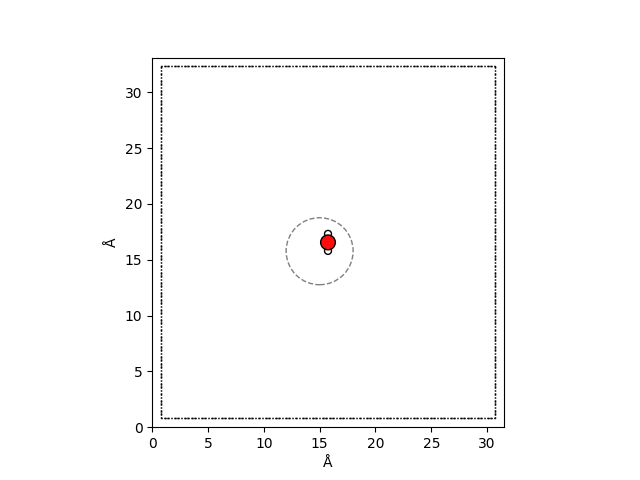
As you can see, for a single water molecule, the cutoff includes all atoms of the
system. The combination of the test system and the cutoff aims to demonstrate that
the full atomic fingerprint is contained within the cutoff. By later subtracting
the short-range density from the LODE density, we will observe that the difference
between them is almost zero, indicating that a single water molecule is a short-range
system.
To start this construction we choose a high potential exponent to emulate the rapidly decaying LODE density and mimic the polar-polar interactions of water.
potential_exponent = 3
We now define some typical hyperparameters to compute the spherical expansions.
max_radial = 5
max_angular = 1
atomic_gaussian_width = 1.2
center_atom_weight = 1.0
We choose a relatively low spline accuracy (default is 1e-8) to achieve quick
computation of the spline points. You can increase the spline accuracy if required,
but be aware that the time to compute these points will increase significantly!
spline_accuracy = 1e-2
As a projection basis, we don’t use the usual GtoBasis which is commonly used for short range descriptors.
Instead, we select the MonomialBasis which
is the optimal radial basis for the LODE descriptor as discussed in Huguenin-Dumittan
et al.
basis = MonomialBasis(cutoff=cutoff)
For the density, we choose a smeared power law as used in LODE, which does not decay
exponentially like a Gaussian density
and is therefore suited to describe long-range interactions between atoms.
density = LodeDensity(
    atomic_gaussian_width=atomic_gaussian_width,
    potential_exponent=potential_exponent,
)
To visualize this we plot density together with a Gaussian density
(gaussian_density) with the same atomic_gaussian_width in a log-log plot.
radial_positions = np.geomspace(1e-5, 10, num=1000)
gaussian_density = GaussianDensity(atomic_gaussian_width=atomic_gaussian_width)

plt.plot(radial_positions, density.compute(radial_positions), label="LodeDensity")
plt.plot(
    radial_positions,
    gaussian_density.compute(radial_positions),
    label="GaussianDensity",
)


positions_indicator = np.array([3.0, 8.0])
plt.plot(
    positions_indicator,
    2 * positions_indicator**-potential_exponent,
    c="k",
    label=f"p={potential_exponent}",
)

plt.legend()

plt.xlim(1e-1, 10)
plt.ylim(1e-3, 5e-1)

plt.xlabel("radial positions / Å")
plt.ylabel("atomic density")

plt.xscale("log")
plt.yscale("log")
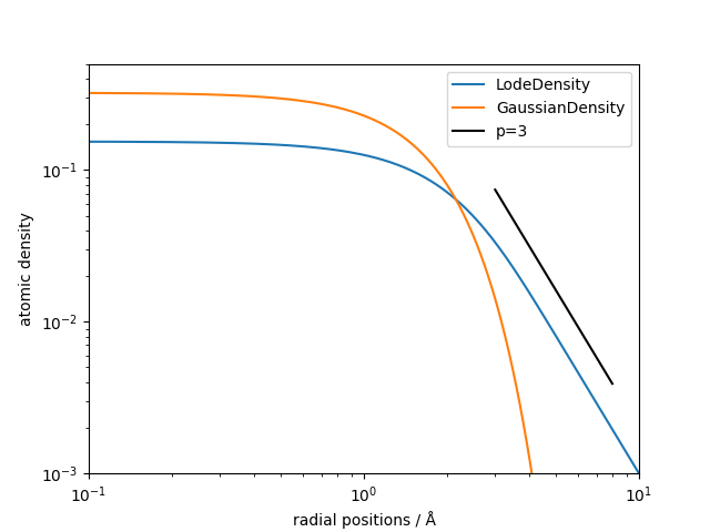
We see that the LodeDensity decays with a power law of 3, which is the potential
exponent we picked above, wile the Gaussian density decays exponentially and is therefore not suited
for long-range descriptors.
We now have all building blocks to construct the spline points for the real and Fourier space spherical expansions.
real_space_splines = SoapSpliner(
    cutoff=cutoff,
    max_radial=max_radial,
    max_angular=max_angular,
    basis=basis,
    density=density,
    accuracy=spline_accuracy,
).compute()


# This value gives good convergences for the Fourier space version
k_cutoff = 1.2 * np.pi / atomic_gaussian_width

fourier_space_splines = LodeSpliner(
    k_cutoff=k_cutoff,
    max_radial=max_radial,
    max_angular=max_angular,
    basis=basis,
    density=density,
    accuracy=spline_accuracy,
).compute()
Note
You might want to save the spline points using json.dump() to a file and
load them with json.load() later without recalculating them. Saving them is
especially useful if the spline calculations are expensive, i.e., if you increase
the spline_accuracy.
With the spline points ready, we now compute the real space spherical expansion
real_space_calculator = SphericalExpansion(
    cutoff=cutoff,
    max_radial=max_radial,
    max_angular=max_angular,
    atomic_gaussian_width=atomic_gaussian_width,
    radial_basis=real_space_splines,
    center_atom_weight=center_atom_weight,
    cutoff_function={"Step": {}},
    radial_scaling=None,
)

real_space_expansion = real_space_calculator.compute(atoms)
where we don’t use a smoothing cutoff_function or a radial_scaling to ensure
the correct construction of the long-range only descriptor. Next, we compute the
Fourier Space / LODE spherical expansion
fourier_space_calculator = LodeSphericalExpansion(
    cutoff=cutoff,
    max_radial=max_radial,
    max_angular=max_angular,
    atomic_gaussian_width=atomic_gaussian_width,
    center_atom_weight=center_atom_weight,
    potential_exponent=potential_exponent,
    radial_basis=fourier_space_splines,
    k_cutoff=k_cutoff,
)

fourier_space_expansion = fourier_space_calculator.compute(atoms)
As described in the beginning, we now subtract the real space LODE contributions from
Fourier space to obtain a descriptor that only contains the contributions from atoms
outside of the cutoff.
subtracted_expansion = fourier_space_expansion - real_space_expansion
combination with a short-range descriptor like
rascaline.SphericalExpansion for your machine learning models. We now
verify that for our test atoms the LODE spherical expansion only contains
short-range contributions. To demonstrate this, we densify the
metatensor.TensorMap to have only one block per "center_type" and
visualize our result. Since we have to perform the densify operation several times in
thi show-to, we define a helper function densify_tensormap.
def densify_tensormap(tensor: TensorMap) -> TensorMap:
    dense_tensor = tensor.components_to_properties("o3_mu")
    dense_tensor = dense_tensor.keys_to_samples("neighbor_type")
    dense_tensor = dense_tensor.keys_to_properties(["o3_lambda", "o3_sigma"])

    return dense_tensor
We apply the function to the Fourier space spherical expansion
fourier_space_expansion and subtracted_expansion.
fourier_space_expansion = densify_tensormap(fourier_space_expansion)
subtracted_expansion = densify_tensormap(subtracted_expansion)
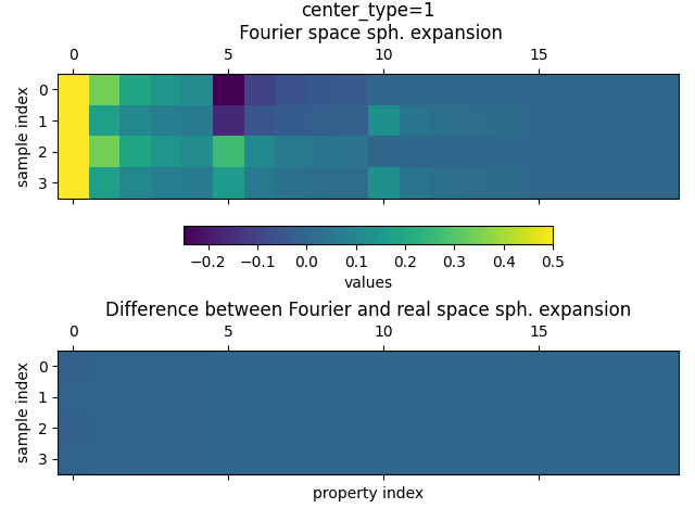
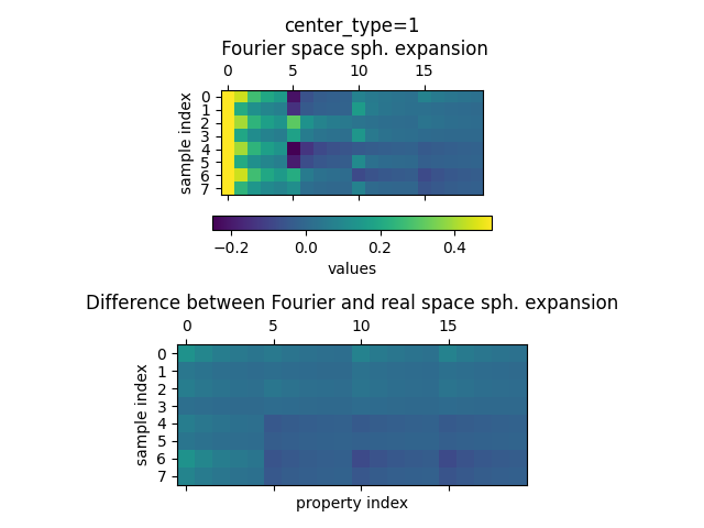
Finally, we plot the values of each block for the Fourier Space spherical expansion in the upper panel and the difference between the Fourier Space and the real space in the lower panel. And since we will do this plot several times we again define a small plot function to help us
def plot_value_comparison(
    key: LabelsEntry,
    fourier_space_expansion: TensorMap,
    subtracted_expansion: TensorMap,
):
    fig, ax = plt.subplots(2, layout="tight")

    values_subtracted = subtracted_expansion[key].values
    values_fourier_space = fourier_space_expansion[key].values

    ax[0].set_title(f"center_type={key.values[0]}\n Fourier space sph. expansion")
    im = ax[0].matshow(values_fourier_space, vmin=-0.25, vmax=0.5)
    ax[0].set_ylabel("sample index")

    ax[1].set_title("Difference between Fourier and real space sph. expansion")
    ax[1].matshow(values_subtracted, vmin=-0.25, vmax=0.5)
    ax[1].set_ylabel("sample index")
    ax[1].set_xlabel("property index")

    fig.colorbar(im, ax=ax[0], orientation="horizontal", fraction=0.1, label="values")
We first plot the values of the TensorMaps for center_type=1 (hydrogen)
plot_value_comparison(
    fourier_space_expansion.keys[0], fourier_space_expansion, subtracted_expansion
)
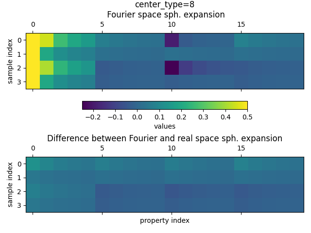
and for center_type=8 (oxygen)
plot_value_comparison(
    fourier_space_expansion.keys[1], fourier_space_expansion, subtracted_expansion
)
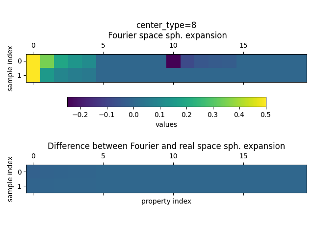
The plot shows that the spherical expansion for the Fourier space is non-zero while the difference between the two expansions is very small.
Warning
Small residual values may stems from the contribution of the periodic images. You
can verify and reduce those contributions by either increasing the cell and/or
increase the potential_exponent.
Two water molecule (long range) system
We now add a second water molecule shifted by \(3\,\mathrm{Å}\) in each direction from our first water molecule to show that such a system has non negliable long range effects.
atoms_shifted = molecule("H2O", vacuum=10, pbc=True)
atoms_shifted.positions = atoms.positions + 3

atoms_long_range = atoms + atoms_shifted


fig, ax = plt.subplots()

ase.visualize.plot.plot_atoms(atoms_long_range, ax=ax)

cutoff_circle = plt.Circle(
    xy=atoms[0].position[1:],
    radius=cutoff,
    color="gray",
    ls="dashed",
    fill=False,
)

cutoff_circle_shifted = plt.Circle(
    xy=atoms_shifted[0].position[1:],
    radius=cutoff,
    color="gray",
    ls="dashed",
    fill=False,
)

ax.add_patch(cutoff_circle)
ax.add_patch(cutoff_circle_shifted)

ax.set_xlabel("Å")
ax.set_ylabel("Å")

fig.show()
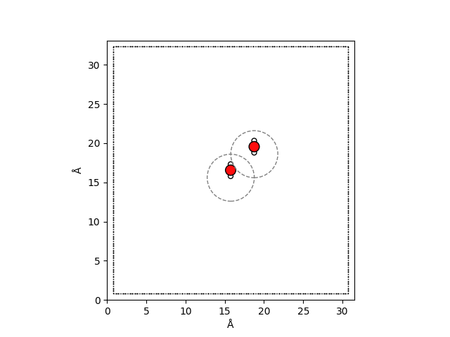
As you can see, the cutoff radii of the two molecules are completely disjoint.
Therefore, a short-range model will not able to describe the intermolecular
interactions between our two molecules. To verify we now again create a long-range
only descriptor for this system. We use the already defined
real_space_expansion_long_range and fourier_space_expansion_long_range
real_space_expansion_long_range = real_space_calculator.compute(atoms_long_range)
fourier_space_expansion_long_range = fourier_space_calculator.compute(atoms_long_range)
We now firdt verify that the contribution from the short-range descriptors is the same as for a single water molecule. Exemplarily, we compare only the first (Hydrogen) block of each tensor.
print("Single water real space spherical expansion")
print(np.round(real_space_expansion[1].values, 3))

print("\nTwo water real space spherical expansion")
print(np.round(real_space_expansion_long_range[1].values, 3))
Single water real space spherical expansion
[[[-0.267 -0.101 -0.06  -0.044 -0.035]
  [ 0.     0.     0.     0.     0.   ]
  [ 0.     0.     0.     0.     0.   ]]

 [[ 0.267  0.101  0.06   0.044  0.035]
  [ 0.     0.     0.     0.     0.   ]
  [ 0.     0.     0.     0.     0.   ]]]

Two water real space spherical expansion
[[[-0.267 -0.101 -0.06  -0.044 -0.035]
  [ 0.     0.     0.     0.     0.   ]
  [ 0.     0.     0.     0.     0.   ]]

 [[ 0.267  0.101  0.06   0.044  0.035]
  [ 0.     0.     0.     0.     0.   ]
  [ 0.     0.     0.     0.     0.   ]]

 [[-0.267 -0.101 -0.06  -0.044 -0.035]
  [ 0.     0.     0.     0.     0.   ]
  [ 0.     0.     0.     0.     0.   ]]

 [[ 0.267  0.101  0.06   0.044  0.035]
  [ 0.     0.     0.     0.     0.   ]
  [ 0.     0.     0.     0.     0.   ]]]
Since the values of the block are the same, we can conclude that there is no
information shared between the two molecules and that the short-range descriptor is
not able to distinguish the system with only one or two water molecules. Note that the
different number of samples in real_space_expansion_long_range reflects the fact
that the second system has more atoms then the first.
As above, we construct a long-range only descriptor and densify the result for plotting the values.
subtracted_expansion_long_range = (
    fourier_space_expansion_long_range - real_space_expansion_long_range
)

fourier_space_expansion_long_range = densify_tensormap(
    fourier_space_expansion_long_range
)
subtracted_expansion_long_range = densify_tensormap(subtracted_expansion_long_range)
As above, we plot the values of the spherical expansions for the Fourier and the
subtracted (long range only) spherical expansion. First for hydrogen
(center_species=1)
plot_value_comparison(
    fourier_space_expansion_long_range.keys[0],
    fourier_space_expansion_long_range,
    subtracted_expansion_long_range,
)
amd second for oxygen (center_species=8)
plot_value_comparison(
    fourier_space_expansion_long_range.keys[1],
    fourier_space_expansion_long_range,
    subtracted_expansion_long_range,
)
We clearly see that the values of the subtracted spherical are much larger compared to the system with only a single water molecule, thus confirming the presence of long-range contributions in the descriptor for a system with two water molecules.